Built up allocation
The principal aim is to estimate the population per grid cell through to the year 2100, commencing with modelling built-up areas and subsequently populating these areas based on suitability scores alongside regional and distributional constraints. Reference built-up land is based on the 2023 release of the GHSL.
To repeat the introductory section in this wiki, the approach to model built-up development is based on four premises: 1) mirroring GHSL assumptions, built-up fractions cannot be reduced, so that only additional built-up fractions are distributed; 2) locations differ in suitability, and more suitable locations are more likely to receive additional built-up; 3) from GHSL built-up grids follows that 60% is a realistic cut-off for built-up development in a grid cell; 4) over time, the statistical distribution of built-up values is remarkably resilient, maintaining similarity to a power-law distribution even in territories with considerable built-up development.
Distributing built-up area
The total area of built-up land that is _added _in a decade is assumed to be known for regions. In the reference application, these regions are so-called functional areas. The built-up allocator described here serves to downscale the exogenous built-up land change and add it to pre-existing built-up land. The currently used GHSL data discerns built-up land with residential and non-residential use. In the reference application, only residential developments are added to the total built-up land that existed in 2020. Model setup is a compromise that makes the best of available methods given limited data and computational resources. The introduced modelling logic aims for the regionally projected new development to be located in the most likely locations while maintaining built-up value distributions close to historical value distributions. This setup is especially limited because the available built-up data is unsuitable for grid-based comparisons over time. Statistical methods are more reliable when assessing land use’s static presence than fractions’ changes. The model setup, therefore, multiplies the results of two empirical elements (namely, estimated suitabilities and an expected top-up) with a counterbalancing mechanism so that the equation is
Weight = % Suitability * Moving-up probability * Balancing factor.
Weight is subsequently used as a proxy to guide the downscaling in a straightforward scalesum() operation, ie scalesum(Weight, identification grid of functional area membership, built-up development at the functional area level)
Allocation of built-up area
Suitabilities
The percentage suitability for the built-up area is determined using a logistic regression analysis performed by the Vrije Universiteit Amsterdam. This logistic regression explains the presence of grid cells at least 2.5% built-upon. In this study, this is referred to as the Calibration. The resulting coefficients per attributing factor are combined with the geographical data of these factors to generate a map that shows the unscaled suitability values of built-up areas being present. Subsequently, this is transformed using a logit function to express the percentage suitability or probability of the built-up area being present. Results from a calibration exercise are shown in Table 1.
Table 1 Exemplary calibration results
| Variables | Africa | Asia | Australia Oceania | Europe | North America | South America |
|---|---|---|---|---|---|---|
| Intercept | 1.759 | 0.310 | 7.393 | -4.620 | 2.761 | 1.674 |
| ln_PopulationDensity_2000_8dir | 0.706 | 0.846 | 1.090 | 1.754 | 0.865 | 1.604 |
| Distance2Coastline | -0.004 | -0.003 | -0.015 | -0.003 | -0.008 | -0.016 |
| Distance2LargeInlandWater | -0.003 | 0.001 | -0.005 | -0.002 | -0.004 | -0.004 |
| Distance2MajorRoads | -0.003 | -0.013 | -0.008 | -0.036 | -0.017 | |
| Distance2SecundaryRoads | -0.005 | 0.001 | -0.004 | -0.003 | -0.006 | 0.008 |
| gc_cities | -0.009 | -0.011 | -0.020 | -0.004 | -0.010 | -0.016 |
| gc_towns | -0.008 | -0.012 | -0.012 | |||
| gc_villages | -0.070 | -0.010 | -0.011 | -0.042 | -0.037 | -0.018 |
| Elevation | 0.0004 | -0.0004 | -0.001 | -0.001 | 0.0004 | 0.0002 |
| slope | -0.022 | -0.150 | -0.035 | |||
| TRI_mean | -1.458 | -1.941 | -2.110 | -0.446 | -1.566 | -1.486 |
| IsProtectedArea | -0.204 | -0.170 | -0.415 | -0.193 | ||
| IsFloodProneArea_RP100 | -0.165 | 0.128 | 0.667 | |||
| Earthquakes_MMI_Index | 0.084 | 0.055 | -0.113 | 0.020 | -0.022 | -0.131 |
| Landslide_prone | -0.206 | -0.067 | -1.049 | -0.455 | -0.352 | -0.198 |
Note: for the most recent calibration results, please refer to the repository or report.
From these results follows that built-up presence is, for instance, more likely with more people in the direct neighbourhood (described by ln_PopulationDensity_2000_8dir), less likely farther from the coast (Distance2Coastline), and less likely in locations with steep slopes (slope). Comprehensive suitability results for Nicaragua are shown in the picture below:
Figure 1 Exemplary suitability map 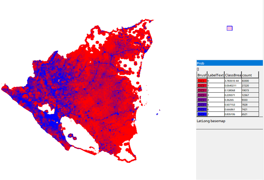
The raw suitabilities for built-up land are calculated in /Analysis/Future/Allocate_Builtup/[YEAR]/Suitability/Calc. Whether these results are recalculated in a model run depends on a model parameter setting. This model parameter can be adjusted as an environment variable when running the model as a batch, or defaults to a value through /ModelParameters/Use_TempTifFiles_manually.
- If
/ModelParameters/Use_TempTifFilesis FALSE, the model will use the results in/Analysis/Future/Allocate_Builtup/[YEAR]/Suitability/Write_Calcand simultaneously store them on the hard drive. This guarantees that the suitability results are consistent with all other model assumptions. - If
/ModelParameters/Use_TempTifFilesis TRUE, the model will read already present suitability results from the hard drive. This is much faster.
Balancing factor
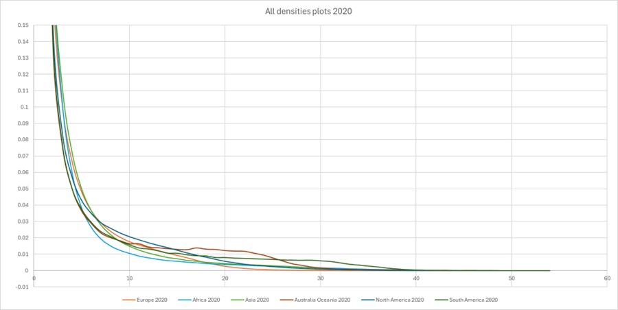
As noted before, the statistical value distribution of built-up land is remarkably resilient and somewhat resembles a power-law distribution. To establish this, built-up fractions from GHSL have been binned into 1%-wide classes in 1990 and 2020, and subsequently plotted for the six continents accounted for (see Figure 2).
Figure 2 Density plots of built-up development by 1% built-up class for all continents 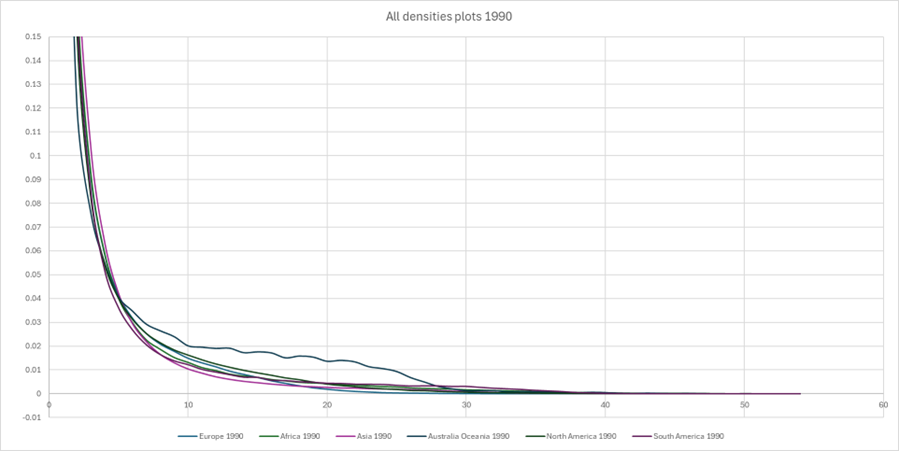
The modelling framework attempts to reflect the resilience of distribution through a set of rules. Cells in the low development range tend to have structurally very low suitabilities. Figure 3 shows the distribution of suitability values, per 1% built-up bin, for Nicaragua.
Figure 3 Suitability distribution by prior built-up class in Nicaragua 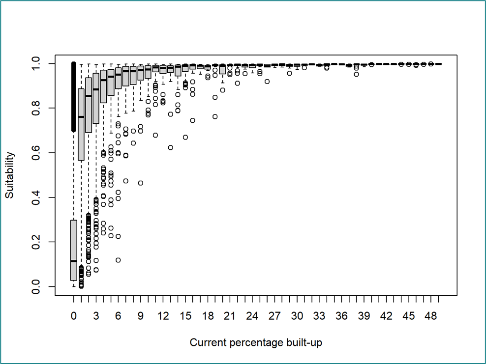
The skewed suitability distribution implies that cells with low prior development would receive very little additional development if the model downscales using unmodified suitability levels as a proxy. This would shift the value distribution to the right and ultimately choke development somewhat as the supply of mid-level development dries up. A counterbalancing mechanism has been introduced to account for structural variation in suitability per level of pre-existing development. This mechanism uses the reciprocal of the average suitability per built-up percentage class to offset the correlation between suitabilities and existing densities. The result is a balanced suitability. Practically, this operation tends to give a bump to suitabilities for grid cells with low prior development levels (see Figure 4).
Figure 4 Balanced suitability distributions by prior built-up level in Nicaragua 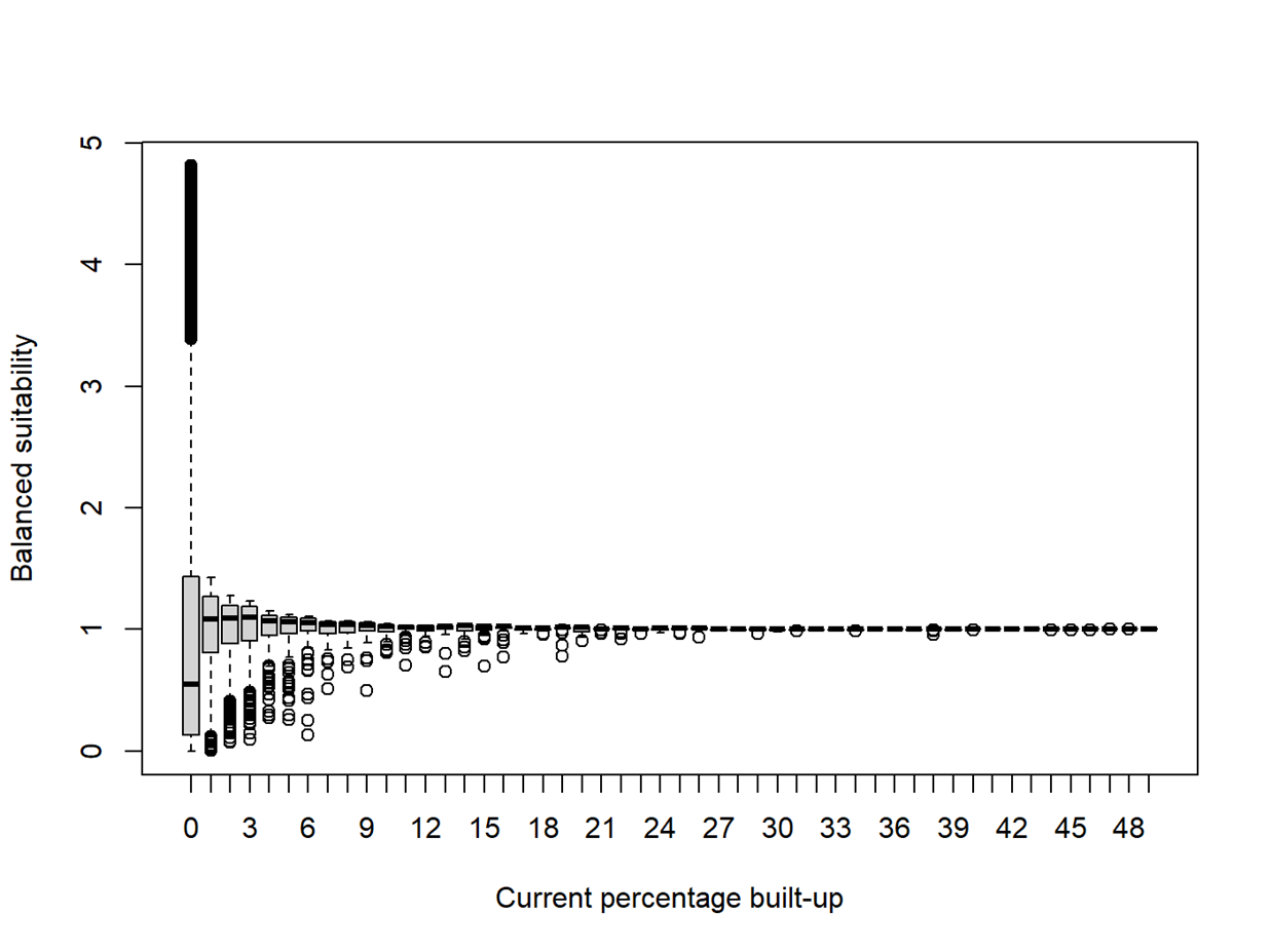
The balanced suitability factor is reproducible through /Analysis/Future/Allocate_Builtup/[YEAR]/Suitability/ProbBalanceFactor.
Expected Top-ups
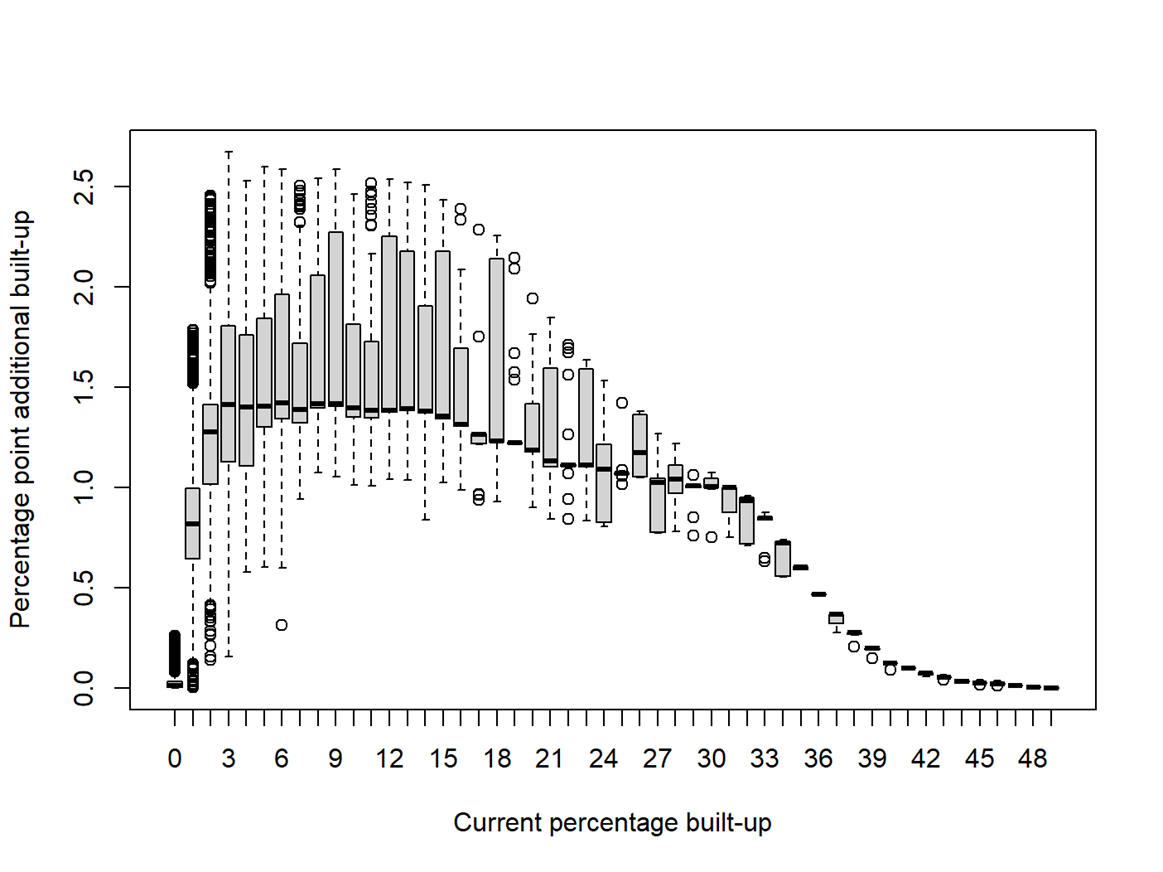
Prior levels of development affect the amount of further development. Critical infrastructure needs to be improved at very low densities, making new development relatively costly. At high densities, development is restricted in terms of available space (and thus degrees of freedom in construction design) and, for example, because of NIMBYism. It therefore stands to reason that the amount of built-up already present in a grid cell has a sizeable impact on the likelihood of further development, and that this impact is decidedly non-linear.
By design, the logit-based suitability functions, such as those used in this study, cannot extract information on how pre-existing development in a grid cell affects further development. More intricate calibration strategies that explain the level of built-up development could take this into account, but are challenged by the fact that observed changes at the grid cell level may be unreliable, and change models generally offer less accurate estimates. Thus, the suitability estimation exercise excludes the value distribution as an explanatory variable.
To include this in the overall modelling framework, Expected Top-ups (ET) factors have been included in the model. These have been computed by first creating transition matrices from built-up percentages in one decade to the built-up percentages in the next decade. Subsequently, ETs were obtained by averaging the additional decennial built-up fractions per built-up percentage class. Some manual smoothing has been applied to take out erratic behaviour in the distribution tails. These ETs are established for all continents, and continent-specific ETs are applied in the current implementation. The currently implemented ETs are shown in Figure 5.
Figure 5: Currently implemented continent-specific ET values 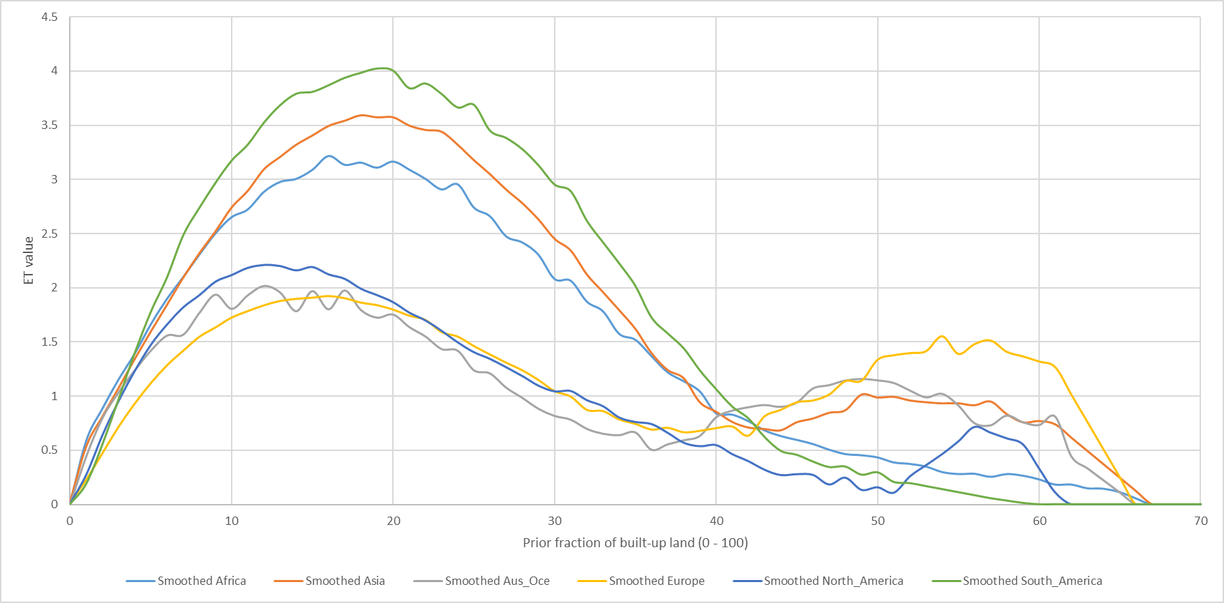
The methods to generate study-area-specific transition matrices are available in /sourcedata/Builtup/percentage_matrix. The currently implemented ET values are available in /Classifications/AllShares and unioned to a generic matrix in /Classifications/Shares_Per_Continent/Moving_up_probability. ETs are computed iteratively in e.g. /Analysis/Future/Allocate_Builtup/[YEAR]/Suitability/Expected_increase, and multiplied with suitabilities and the balancing factor discussed below in /Analysis/Future/Allocate_Builtup/[YEAR]/Suitability/FinalProb. The algorithm foresees an optional weighting of ET values, by which ETs in a territory are weighted with the available space in the territory. This leads to relatively more transitions towards high built-up fractions in regions with limited space availability. The weighting approach is coded in /Analysis/Future/Allocate_Builtup/[YEAR]/Suitability/Dynamic_Expected_increase.
The final proxy by which additional built-up area is downscaled is then finally calculated by multiplying the initial probability from calibration, the suitability rebalancing factor, and the ET value. The distributional results of this multiplication are given in Figure 6 for Nicaragua as a graph. This graph shows that the combination of locational suitabilities, rebalancing and ETs creates a rich pattern of outcomes with particularly strong variation in low development classes where ETs are high and locational suitability varies considerably.
Figure 6 Distribution of the proxy variable used for downscaling built-up in Nicaragua 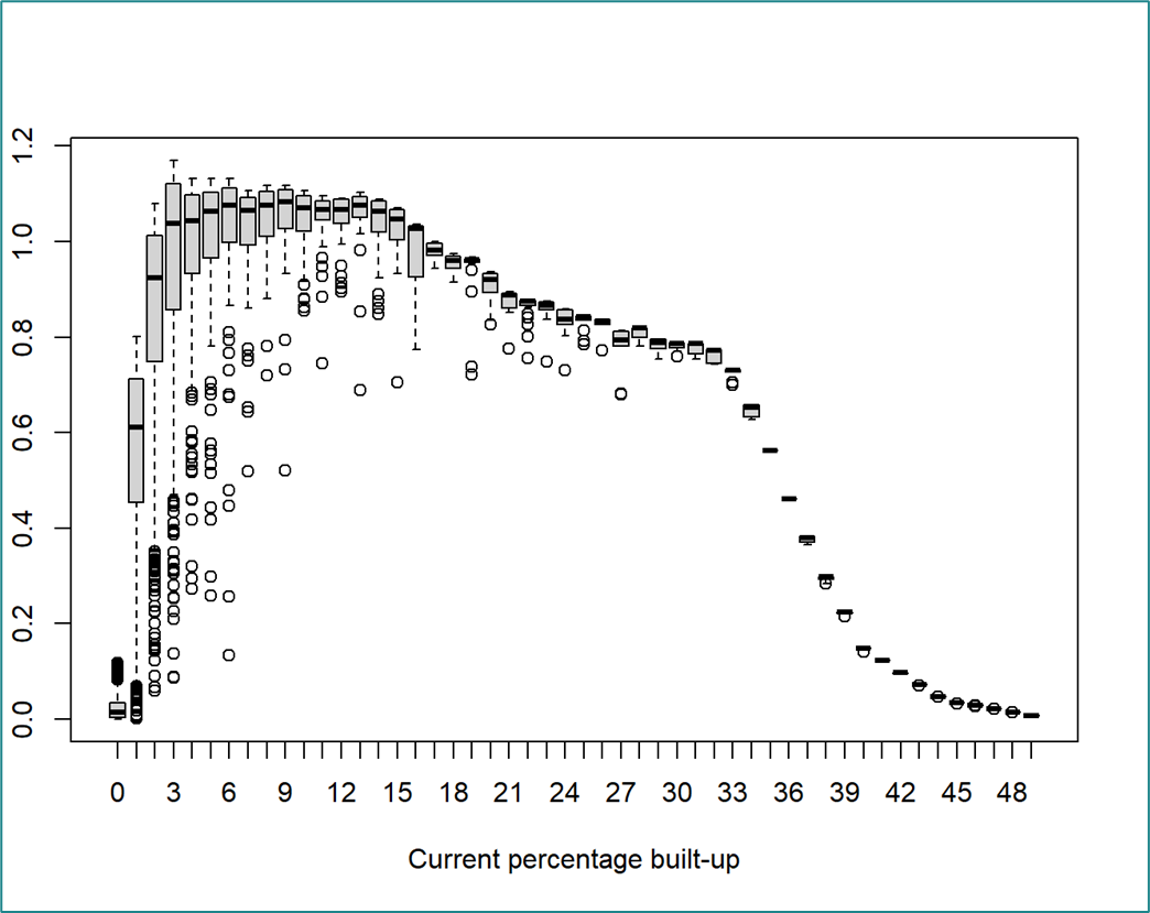
Note: in the reference application, a dynamic version of the Expected Top-ups is being utilised. This entails a modified version of the empirically obtained ET values in which these values respond to the amount of space in a functional area that is still available for built-up development. Effectively, this modification causes ETs on the right-hand side (and subsequently built-up densities) to increase somewhat where space for development is limited. This is explained further in the section Dynamic expected top‐ups
Allocation procedure
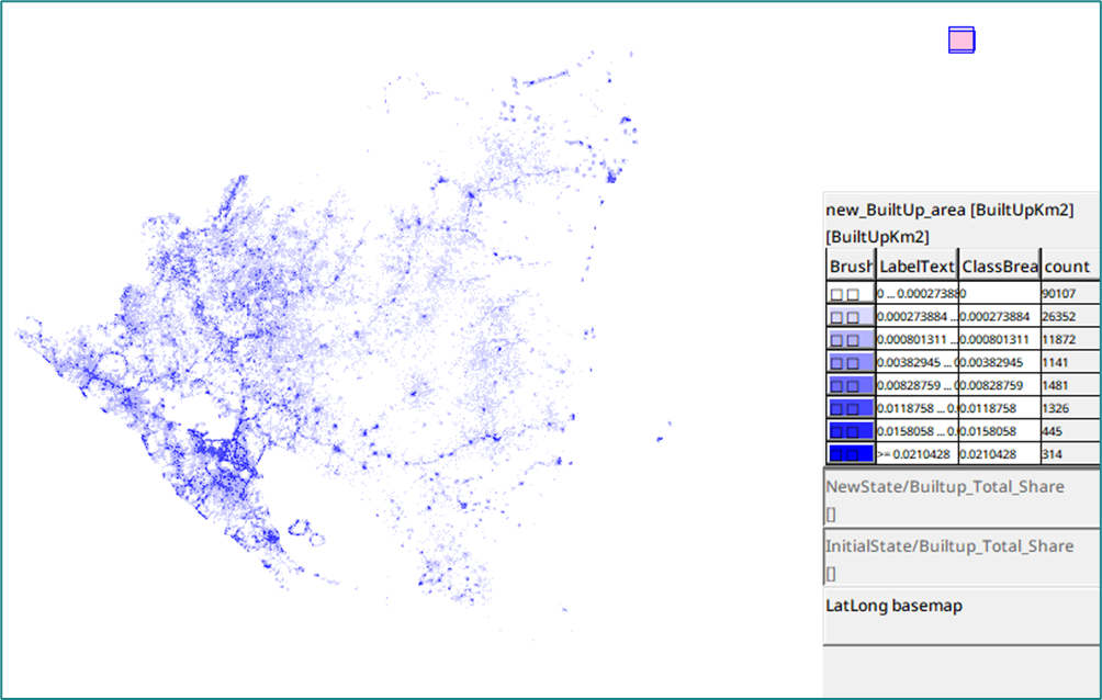
The final probability for the built-up area is subsequently used as a proxy to disperse the remaining regional claims. The regional claim is subsequently mapped dasymetrically using a weighted scalesum() operation in /Analysis/Future/Allocate_Builtup/[YEAR]/NewState/new_BuiltUp_area_raw. The result of this downscaling is shown graphically and geographically in Figure 7 for the case of Nicaragua.
Figure 7 Exemplary built-up allocation results for Nicaragua