Geography
The model at hand is geographically explicit and therefore depends critically on a number of definitions of geographic space. This section goes into more detail about how geographies are described and delineated in the model.
Geography in model mechanics
Projection systems
The model can run in two separate projection systems, namely in WGS84 (‘latlong’) and Mollweide equal area (‘Mollweide’). Mollweide equal area is used in the reference projections to ensure consistent estimates of degrees of urbanisation, as those depend on equivalent neighbourhood sizes across the globe. Which projection system is run is governed through /ModelParameters/domain_EPSG. If that parameter is set to ‘54009’, the projection system is Mollweide; else it is WGS84. Do note that the choice of projection system also requires, e.g. sourcedata and estimated parameters from Calibration (a recent calibration exercise has provided parameters for models in both projection systems).
Study areas
Because of memory limits, the model cannot be run for the entire globe in one go. Thus, a study area needs to be defined in order to confine the model. This study area needs to be a continent or country as named with a parameter in /sourcedata/RegionalUnits/Continents/V or /sourcedata/RegionalUnits/Countries/V respectively. To change the study area, adapt /ModelParameters/StudyArea_manually. This is a manual setting; study areas can also be changed through an environment variable when accessing the model through a DOS batch file and GeoDMSrun.exe. A large number of study area definitions are already available for both Mollweide and LatLong in /Geography/StudyAreas. If a wanted study area is not yet defined, users can add it by copying and pasting and then adapting the code in that model section.
Compacted domain
The model derives its observations and most data from tiled rasters. These rasters are designated as ‘domain’ (internal reference is /geography/domain). For the sake of computational simplicity, the model does not include all grid cells within a study area. We exclude grid cells that
- are not within the territorial boundaries for which exogenous expectations on built-up and population are defined;
- are permanently covered by surface water or ice; and
- are more than 5km away from a grid cell that has any built-up development in 2020.
The resulting selection of grid cells that are included in the modelling is called the ‘compacted domain’. This domain is defined here: /geography/domain_Mollweide/IsCompactedDomain
The boundaries-based criterion ensures that grid cells are not somehow included if they are not covered in the exogenous regional projections for built-up and population. We exclude grid cells permanently covered by water and ice, as sustained built-up development is highly unlikely in such locations (thus, we are not taking into account efforts to reclaim land from water). Finally, we exclude all grid cells that are more than 5km away from any known built-up development estimated by GHSL built-up for 2020. This criterion was chosen to restrict the number of observations used for modelling in land areas with very limited human occupation, such as the Sahara Desert. Historical analysis shows that, between 1975 and 2020, a negligible amount of built-up development occurred at places that were more than 5km away from a grid cell that had some built-up land in 1975. We therefore think that this selection for optimisation does not negatively affect modelling outcomes by cutting out plausible locations for built-up development. As an example, the grid cells included in the compacted domain (1) and the unselected cells in the tiled raster domain (0) are shown for Africa in Figure 1.
Figure 1: Result of selecting the compacted domain in Africa, based on the criteria outlined in this section 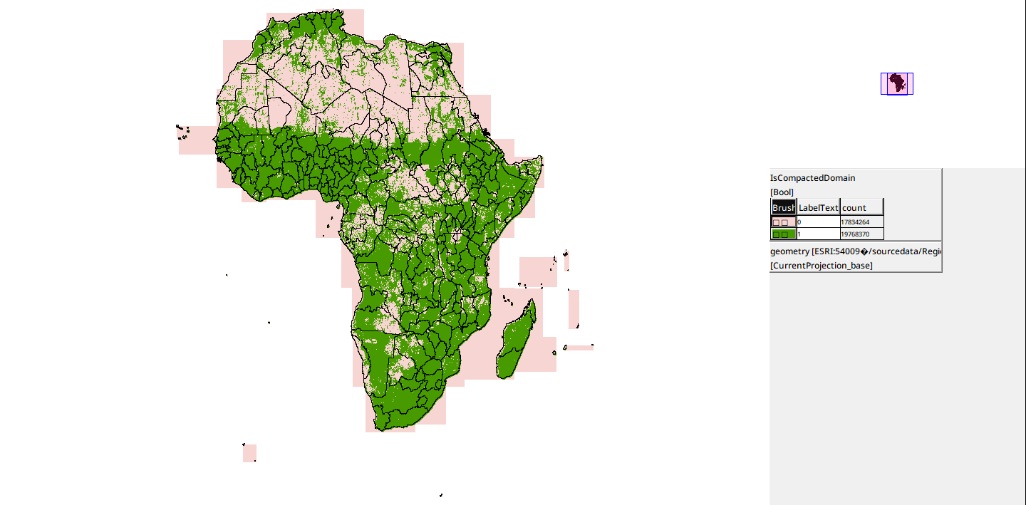
Internally used boundaries
The model uses a set of internal boundaries that represent continents /sourcedata/RegionalUnits/Continents, countries /sourcedata/RegionalUnits/Countries and subnational units within countries /sourcedata/RegionalUnits/FunctionalAreas_all. These internal boundaries represent the best set of boundaries available for our modelling purposes, but do not represent a position on existing border conflicts or contested areas. All internal boundaries derive from the so-called functional areas as explained in the section that describes how we Define subnational units for projections. The countries and continents we use are recreated by the dissolving (or union) of functional areas into larger landmasses.
Many of the choices in the model’s internal boundary system thus cascade from choices made in the functional area creation process. The source of all country borders is the GADM database. However, these borders have been adapted by JRC’s GHSL team, essentially moving country boundaries 3km into seas and oceans where possible. This has the advantage that, e.g. outcrop raster cells are always included within country borders. Another important change is that, for modelling purposes, the Russian Federation has been split into a European and Asian part named ARUS and ERUS. This has been necessary because the functional area definitions depend on the continental OpenStreetMap (OSM) network databases. In those OSM databases, Russia is also split into a European and an Asian part. The model inherited this separation, so that Russia is split into two ‘countries’ that are on different continents. Figure 2 shows the current representation of continents in the model, highlighting Europe.
Figure 2: Continents as they are currently defined in the CRISP model 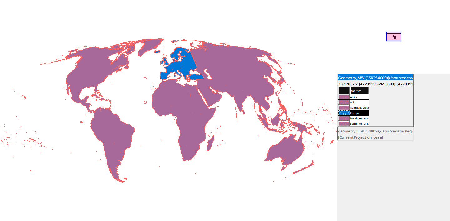
Neighbourhood definition
Grid neighbourhood definitions are typically defined in GeoDMS through kernel matrices (i.e., /geography/Distmatrices/Impl/pot40km/potRange) and then used in functions applying convolution such as potential(). Many of the neighbourhood operations in the model at hand are a break from this practice. We often do not define a distance matrix, which is a combination of the compacted domain and a distance-based kernel. Using this approach reduces memory requirements, especially in cases in which a study area spans parts of the Western and Eastern hemispheres, e.g. Oceania and Asia. This general modelling improvement is discussed in more detail in https://github.com/ObjectVision/2BURP/issues/44.