Introduction

Expected Top-ups (ETs) are used in the CRISP modelling framework to ensure that prior development levels affect additions of built-up land. These are described in more detail in the section Built up allocation. The ETs are based on transition matrices in which aggregate outcomes in 2000, 2010 and 2020 were aggregated by prior level of development (per 1% built-up bin in the preceding decade). These values reflect the distribution of built-up development given historical, presumably mostly unconstrained increases in aggregate built-up land. The projections applied in the reference application indicate very rapid population growth and even more rapid urbanisation in parts of the world. For some of the functional areas used in the reference application this leads to an absorption of available space that has no historical precedent. In these cases, the empirical ETs would cause entire regions to become developed mostly with mid-range built-up fractions. This seems implausible. The lack of precedent implies that we cannot verify historical responses to space limitations.

Definition

As a project-specific assumption, we therefore modify the ETs with a dynamic component. This dynamic component is based on the amount of space available in a functional area. This is defined in /Analysis/Future/Allocate_Builtup/[YEAR]/Claims/Available_Space as:

Available space = 1 - (Total area expected Built-up in [YEAR] / Area in compacted domain)

Subsequently, weights are computed for every grid cell based on the current fraction of built-up in /Analysis/Future/Allocate_Builtup/[YEAR]/Suitability/Available_Space_Weight as:

Available space weight = (% Current Built-up * 100) / Available space

We derive the original Expected Top-up given continental ET values and the gridcell-specific built-up fraction in /Analysis/Future/Allocate_Builtup/[YEAR]/Suitability/Expected_increase. We then finally modify this expected value with the available space weight so that:

Dynamic ET = (1 + Available space weight) * Expected increase

Interpretation

The dynamic weighting of ET values effectively increases ET values for grid cells with higher prior built-up levels for all cases where the available space is below 1. Figure 1 shows trhe distribution of available space weights for different values of Available space (A).

Figure 1 Available space weights for different levels of prior built-up development (x-axis) and available space (A)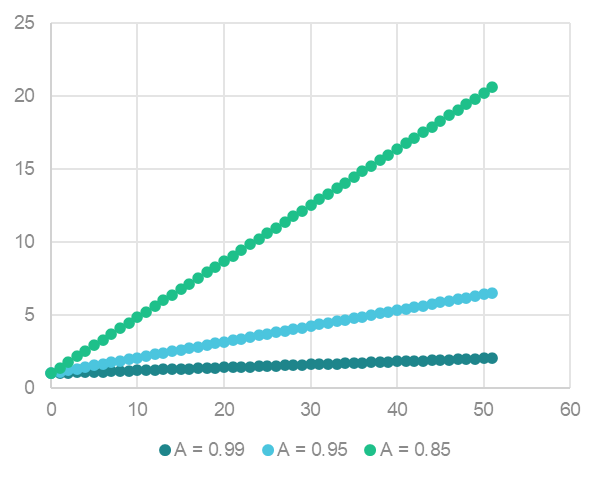

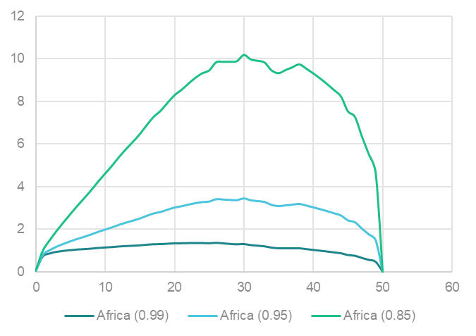
Multiplying ET values with these available space weights causes a notable general value increase, see Figure 2. General value increases do not necessarily affect the downscaling, as the weighted ETs are only used as a proxy variable in a scalesum.

Figure 2 Available space weights multiplied with tentative ET values for Africa

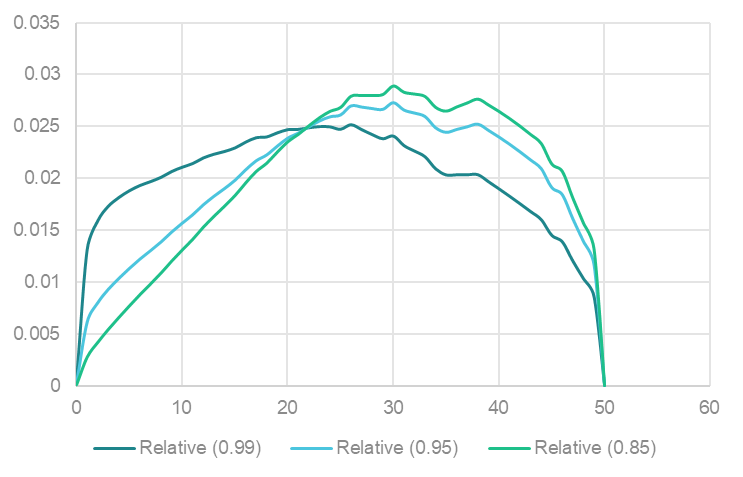
However, the weighting also causes a rearrangement of the distribution. This is more obvious when scaling back the above three weighted distributions, so that for all three lines the sum of all values is 1 (see Figure 3). There clearly the weighting causes increasing emphasis on the right-hand side of the current built-up range. In turn, this nudges the model to concentrate more of the additional built-up development in areas that already have considerable levels of development.

Figure 3 Tentative ET values weighted by available space weights and then rescaled so that the sum of all values in a line is 1