Population allocation
Distributing population
Population is distributed according to stylised, universal rules that depend on 1) the simultaneous results of Built up allocation, 2) the locational suitability functions for built-up land that are estimated in the Calibration exercise, and 3) a number of general time and location-specific limitations. We msut concede that, ideally, the population distribution procedure is tied less stringently to built-up modelling than is currently the case (as discussed e.g. here). To properly capture population changes, data is required that describes ground-truth, observed population changes. Unfortunately, such population data is still elusive at the global level. Available population data such as provided by GHSL are the result of dasymetric mapping that relies on built-up fractions or built-up volume as a proxy. We thus make use of these, and will later explore population changes in more detail in locations where the needed ground-truth population grids are available.
The distribution of the population proceeds in four steps: 1) The initial population is reduced to accommodate population decline and facilitate densification. This reduction approximates migration out of grid cells. The reduced population partially is moved to a functional-area specific population pool. Population is initially taken out of grid cells that are unattractive according to the logit transformation of locational suitabilities. 2) If not enough people can be taken out of unattractive grid cells to obtain the expected number of outmigrants, a blanket percenta of additional people are drawn out of still populated grid cells. 3) Then, the newly built-up areas will be populated based on the average initial built-up population density in the neighbourhood. This neighbourhood is defined using a 3x3 cell radius. 4) The remaining population claim is met by iteratively assigning the population to cells according to suitability with an increasing scaling factor. This assignment is limited by the maximum allowed density.
These steps are designed to allocate newcomers in a functional area and slowly reallocate the population, taking into account declines and the likely slight densification.
GHS-POP data serve as the basis for population modelling, with 2020 as the reference year. However the aggregate populations in 2020 according to the GHSL layer do not match national populations in 2020 according to the population projections used in this study. To eliminate any inconsistencies due to agreement on aggregate population counts, Marcello Schiavina has prepared a tailored set of population grids 1975 - 2020 that are fully consistent with the population totals according to the used projections.
Allocation of population
Population and population density
First, we determine the number of persons per km2 of residential built-up area and truncate this to the maximum of 1 million people per km2 of residential built-up area (or one person per m2). Calculating this back to the number of persons per cell, we corrected discrepancies between the GHS and GHSL data layers.
Local maxima
We start by determining the maximum number of persons per cell that the population may grow in a timestep. A timestep entails a decade, and is noted here as T1 to T2.
As a general rule, the model does not allow population densities to exceed 100,000 inhabitants per km2. Furthermore, the model applies timestep-specific constraints. These constraints are derived from an extensive analysis of historical population changes according to the 2023 release of GHS-POP.
- If a cell has the highest local population in a square of 3x3 in T1, it can only increase by 3,500 people per km2 built-up in T2 (parameter in
/ModelParameters/Pop_r_if_LocalMax); - If a cell is populated but it doesn’t have the highest local population in a square of 3x3 in T1, it can only increase in T2 to the local maximum in T1 + 2,500 people per km2 (parameter in
/ModelParameters/Pop_r_if_notLocalMax); - If a cell is not populated in T1, it can only increase by 350 people per km2 built-up in T2 (parameter in
/ModelParameters/Pop_r_if_notPopulated). These constraints are multiplied with simultaneous built-up fractions; they are grid-cell specific and recomputed in every timestep. The decision tree for these constraints is coded in/Analysis/Future/Allocate_Population/[YEAR]/LocalMaxima/MaxAllowed_Population. Finally all constraints are expressed as room for additional population in e.g./Analysis/Future/Allocate_Population/[YEAR]/NewState/Room_for_Population. This is done by taking the absolute constraint, and reducing it with the population present before allocation.
Filling population pools
Every functional area has a population pool that contains foreseen population growth plus a parametrized percentage of the prior population. This parameter percentage represents internal migration and is adaptable through /ModelParameters/Pop_Internal_Migration_Reduction_Rate_base. In the reference application this internal migration parameter is set at 1%.
- If the regional population increases, the pool size equals the population growth + the portion of the regional population that is set to migrate within the region.
- If the regional population shrinks, a larger portion of the prior population is taken out of grid cells, ensuring that the model reallocates the wanted internal migration rate. In this case the population pool equals the internal migrants.
The percentage of people that needs to be drawn from the grid cells in a functional area is defined in e.g. /Analysis/Future/Allocate_Population/[YEAR]/Initial_Population_Scaled_Reduction_Rate, and computed as such:
Rate to be drawn = minimum(% population change, 0) - Internal Migration Rate
which is subsequently treated as an absolute (ie positive) value and multiplied with the amount of people in T1 in the functional area. The result is the amount of people that needs to be drawn in e.g. /Analysis/Future/Allocate_Population/[YEAR]/NewState/Regional_Population_to_draw
Population is subsequently first taken out of locations weighted by unsuitability. This is done using the results from the logit probability function estimated in Calibration. Using these probabilities we establish the scaled reduction rate /Analysis/Future/Allocate_Population/[YEAR]/Suitability/Scaled_Reduction as:
Scaled reduction = 1 - (0 <= probability <= 1)
Subsequently, we create a proxy variable for reductions in /Analysis/Future/Allocate_Population/[YEAR]/Suitability/Scaled_Reduction_Proxy as :
Reduction proxy = Population (T1) * Scaled reduction
We subsequently compute the amount of people that we draw from each grid cell through a scalesum in /Analysis/Future/Allocate_Population/[YEAR]/NewState/Regional_Scaled_Reduction, limiting the total draw to the amount of people present:
Scaled reduction = scalesum( Reduction proxy, functional area rel, regional population to draw ) <= Population (T1)
The thus realised reduction is capped to ensure that no more people are taken out than present in a cell. In rare cases with sizeable population reductions (or limited population in unsuitable locations) the Regional scaled reduction may not be sufficient to draw sufficient people to the functional area’s population pool. Thus the sum in /Analysis/Future/Allocate_Population/[YEAR]/NewState/Regional_Scaled_Reduction may be smaller than the regional population to draw. To ensure that the population pool is filled sufficiently, we draw the necessary remainder as a percentage of every grid cell’s remaining population. To do so, we first assess the percentage of people that still need to be drawn in /Analysis/Future/Allocate_Population/[YEAR]/NewState/Proportion_Potential_Additional_Reduction. This is done per functional area as:
Proportion of potential additional reduction = (Regional population to draw - Regional scaled reduction) / (Population, T1 - Regional scaled reduction).
We then draw a second group of population from grid cells in /Analysis/Future/Allocate_Population/[YEAR]/NewState/Additional_Proportional_Reduction as:
Additional proportional reduction = Proportion of potential additional reduction * Population (T1)
Subsequently, we identify the remainder population in /Analysis/Future/Allocate_Population/[YEAR]/NewState/Remaining_Population as:
Remaining population = Population (T1) - Scaled reduction - Additional proportional reduction
The below Figure 1 illustrates the potential distribution of reductions from the existing population (T1). In this example, the majority of population reductions is drawn from cells with a low locational suitability. However another 5% of the population is drawn proportionally for the sake of example; practically such a considerable proportional reduction only occurs in functional areas undergoing sizeable population decline.
Figure 1 exemplary scaled and proportional population reductions by stylized locational suitability bins 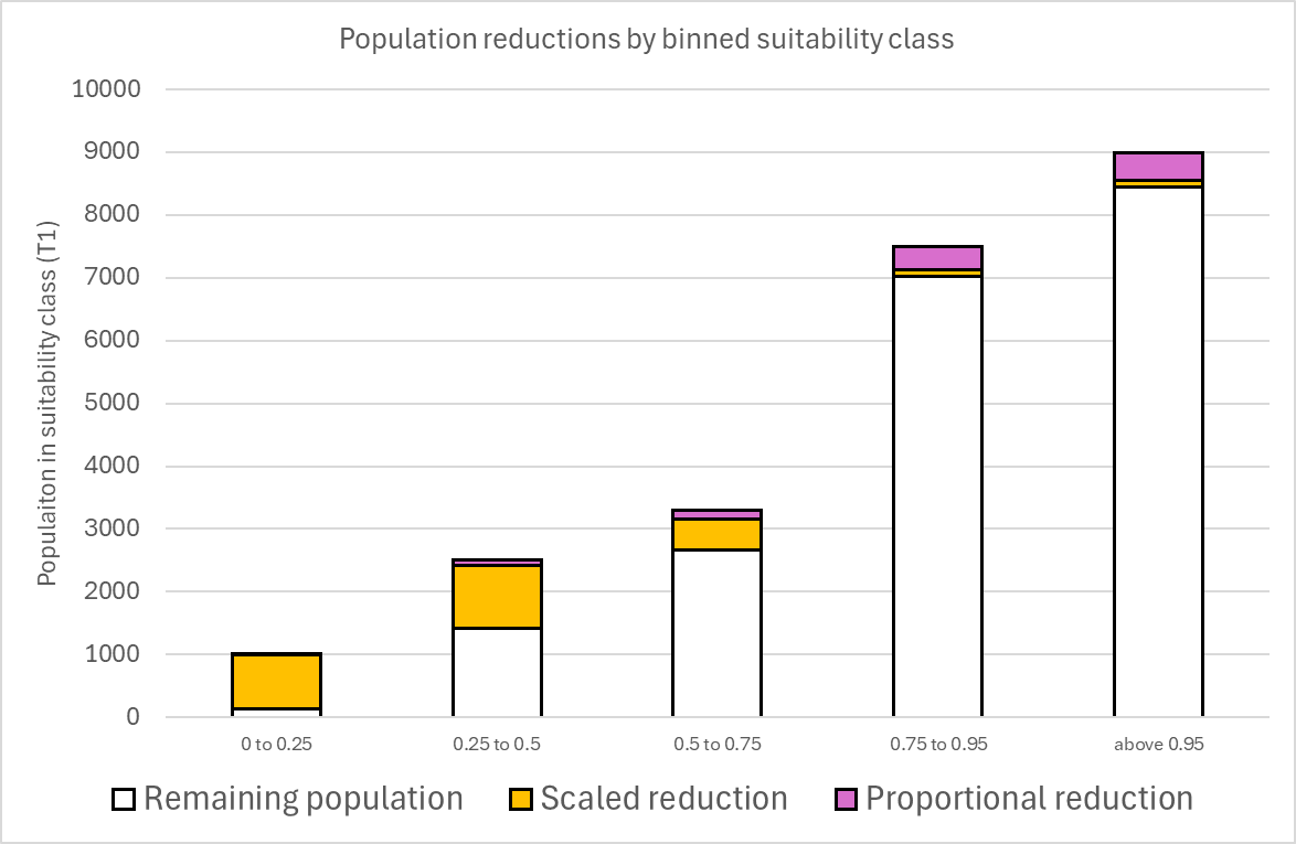
Given the remainder population, we can compute the population pool. This is not done explicitly in the model, but would take this shape:
Regional pool = Expected population in T2 - Remainder population
NOTE: In earlier model versions, the amount of people drawn from unsuitable location also depends on the percentage of a grid cell that we maximally allow to be taken out of a grid cell. This percentage is governed through a parameter, namely /ModelParameters/Pop_Suitability_Reduction_Scale. In the reference application this parameter is set to 0.9 (90%). It is advisable to set this parameter above 0.5, as that allows grid cells to become depopulated. The code has evolved considerably since this parameter was included. At this moment it is unsure if this setting still has an impact on results. This needs to be verified.
Allocating people to new built-up land
Next, we allocate population to newly built-up areas. New built-up areas in T2 are obtained from Built up allocation results in T2, reduced with the built-up results from T1. Thus these represent fractions of built-up land in every grid cell. Grid cells that already were partially built-upon in T1 can still have some The amount of population that a fraction of built-up land receives depends on three factors:
- The amount of people in the regional pool, as discussed in the previous section.
- The parameter
/ModelParameters/Pop_ShareOfRestclaim_Prefers_newBUthat optionally maximizes the share of people in the regional pool allowed to be allocated to new built-up land (in the reference application this parameter is set to 1, so that there is no effective maximization). - Average population over built-up land in the 3x3 neighbourhood.
This is accomplished by first calculating the average local population density in a residential area multiplied by the newly built-up area. The average local population density is calculated through /Analysis/Future/Allocate_Population/[YEAR]/NewState/Avg_Local_Population_inRes_Density and is based on the total population (in T1) and total built-up fractions (in T2) in a 3x3 neighbourhood as:
Population density = Total population (T1) in 3x3 neighbourhood / Total builtup (T2) in 3x3 neighbourhood
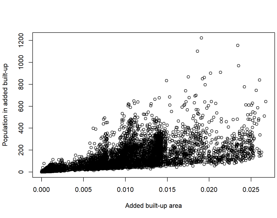
This population density is what can maximally be allocated to a newly developed area. This maximum is scaled down proportionally if necessary, to ensure that the remaining population plus the just allocated population in new built-up areas does not exceed the regional projection, while retaining the geographical variation in population densities stemming from the local population density measure. The resulting additional population is coded in /Analysis/Future/Allocate_Population/[YEAR]/NewState/Population_in_New_BuiltUp_Area and added to the remaining population in /Analysis/Future/Allocate_Population/[YEAR]/NewState/Population_beforeAllocation. In most cases, this has yet to satisfy the regional population projection. Figure 2 shows provisional results for Nicaragua by juxtaposing additional built-up land in a grid cell with the amount of people allocated in a modelling timestep.
Figure 2 Provisional results from a modelling timestep in Nicaragua showing additional population allocated to new built-up land as a function of the amount of built-up land in a grid cell
###Allocating the remainder population while maintaining local constraints Next, an iterative process allocates the regionally projected population proportional to suitability. Simultaneously, constraints are controlled for, ensuring that modelled population does not exceed the previously established local and general maximum population levels. Proportions that are omitted due to the saturation are allocated in subsequent iterations.
To achieve this, we first calculate the remaining vacancy for population per cell, which is the difference between the population from the previous step (ie, /Analysis/Future/Allocate_Population/[YEAR]/NewState/Population_beforeAllocation) and the maximum allowed population per cell (/Analysis/Future/Allocate_Population/[YEAR]/LocalMaxima/MaxAllowed_Population). This yields a grid-specific vacancy level, which we multiply with an indication of the locational suitability of the grid cell. The suitability factor used here differs from the logit probability levels used earlier. Instead we take 1) the absolute suitability values before the logit transformation, ie the added results of multiplying estimated parameters with variable grids; and 2) truncate negative values, so that suitability values are zero or higher (in /Analysis/Future/Allocate_Population/[YEAR]/Suitability/NonNegative).
The product of vacancy and suitability is deemed a proportionality factor, so that:
Proportionality factor = vacancy * ( 0 >= suitability )
This factor is aggregated per region into the ‘summed proportionality factor’ (/Analysis/Future/Allocate_Population/[YEAR]/NewState/Sum_ProportionalityFactor). We then calculate a scale factor by dividing the remaining claim with the summed proportionality factor, ie:
Initial scale factor = Expected population (T2) - Remaining population - population in new built-up land / Summed proportionality factor
This expresses the amount of people to allocate, per unit of proportionality, which in turn is a product of vacancy and suitability.
Subsequently iterations are needed to optimize the distribution of population given proportionality. This iterative process has crude similarities with an iterative proportional fitting procedure. Per iteration, an adapted scale factor is fed into the loop.
Starting from the initial scale factor, 1) proportional population is distributed by multiplying the grid-cell proportionality with the input regional scale factor 2) proportional population is capped so that it does not exceed the vacancy 3) capped proportional population is added to the population never moved and allocated to new built-up areas, yielding realised total population 4) a regional rescaling factor is estimated as the factor difference between wanted, exogenous, regional population and the population realised in this iteration 5) the regional scale factor is multiplied with the rescaling factor, and subsequently passed to the next iteration. The process starts again from 1) with this new factor.
Effectively, this iterative procedure starts by distributing the remainder population over the product of vacancy and suitability. In some places this will cause an overshoot vis-a-vis vacancies. Capping on vacancy means that the input scale factor does not lead to allocation of the entire remainder population. Thus iterative rescaling is needed in which effectively the proportional populations keeps producing larger overshoots, until the subsequent, vacancy-capped population equals the wanted remainder population size.
Transform to integer population count
The result of the iterative pushing upwards, then capping, is an optimized population distribution (given constraints and suitabilities). The result is a population distribution that is equal to the expected population and respects the imposed constraints. However, the population is expressed as a floating number, so that fractions of a person may be present in a grid cell. We subsequently transform these fractions into an integer number of people using a simple workflow: 1) transform the floating population to an integer 2) calculate n as the total population lost after transformation, as sum ( total population ) - sum (integer population ) 3) rank grid cells by the size of the fraction lost because of transformation to integer 4) select the n grid cells with the highest rank from 3) and add a person to each.
This process ensures integer population while maintaining the wanted population totals.